
















Next 30 Days Daily Reservoir Water Level Prediction Using Deep Neural Networks: FNN, GRU, and LSTM Models.
Deep Neural Networks have become powerful tools for businesses, enabling them to simplify complex processes and make informed decisions. These networks help analyze and identify risks, develop effective mitigation strategies, and optimize existing resources to achieve maximum output. Deep neural networks such as GRU and LSTM are excellent in predicting future from the time series data, however, the models are highly dependent on the data quality, parameters and the hyperparameters.

In recent years, Deep Neural Networks have become powerful tools for businesses, enabling them to simplify complex processes and make informed decisions. These networks help analyze and identify risks, develop effective mitigation strategies, and optimize existing resources to achieve maximum output. Their applications extend to various fields, including water resource systems, where they play a critical role in enhancing efficiency and decision-making.
Knowing the future availability of water in a reservoir plays an important role in the effective operational planning of water resources. This information is critical for ensuring the efficient management of water supply distribution systems, optimizing hydropower generation, supporting irrigation practices, and implementing flood control measures. Once the forecasting water levels is done, decision-makers can better allocate resources, enhance system reliability, and address potential challenges in these critical areas.
In this article, I will predict the reservoir water levels for the next 30 days using three deep neural networks: Feedforward Neural Networks (FNN), Gated Recurrent Unit (GRU) and Long and Short Term Memory (LSTM) from a time series data of historical reservoir water level. The analysis is based on 10.5 years of daily reservoir data, evaluating the performance of these models. These three deep neural networks are well-known for their exceptional ability to handle time series data, making them excellent predictors in this domain.
I have a 10 and half years daily data which is nearly 4115 data points. Although using longer recorded data increase the accuracy of the prediction, I only used 10 years data for the simplicity. To start, I used a PyCharm professional with student version so that it can enables me to import necessary libraries including the Jupiter notebook. Let’s start by importing important libraries.
import pandas as pd
import numpy as np
import matplotlib.pyplot as plt
from sklearn.model_selection import train_test_split
from sklearn.preprocessing import MinMaxScaler
from tensorflow.keras.models import Sequential
from tensorflow.keras.layers import Dense, LSTM
from tensorflow.keras.layers import GRU
from sklearn.metrics import mean_absolute_error, mean_squared_error
Pandas and NumPy are used specifically for data manipulation and numerical operations.
Matplotlib is included for visualizing data and used to draw any plots such as charts and model performance.
The train_test_split function from sklearn.model_selection helps in splitting the dataset into training and testing sets. Spliting data into training and testing are important to control how our training is performing.
MinMaxScaler from sklearn.preprocessing scales the data into a normalized range, which is crucial for neural network performance.
Sequential, a framework for creating neural network models, and layers like Dense, LSTM, and GRU from TensorFlow Keras. These layers enable building deep learning models such as Long Short-Term Memory (LSTM) and Gated Recurrent Unit (GRU), both of which are particularly effective for sequential and time-series data.
Mean_absolute_error is used to evaluate the model performance and the accuracy of the predicted values.
Next, Let’s load our data from it’s source. In my case I import the data directly from my computer. However, if you want to use the data to train yourself, you can use my GitHub accout here It’s a CSV file a daily record of 10 years data. However, can use different technique to load your data.
# Load data from the first sheet (Koka)
data = pd.read_excel("cleaned_tekeze.xlsx", sheet_name=0)

# Ensure Date is datetime and sort by Date
data["Date"] = pd.to_datetime(data["Date"], errors='coerce')
data = data.dropna(subset=["Date"])
data = data.sort_values(by="Date")

# Extract useful features
data["Year"] = data["Date"].dt.year
data["Month"] = data["Date"].dt.month
The code above allows us to handle missing data as well as incorrect date and year entries. Since there is no missing data in this dataset, no values will be dropped. Now, let’s visualize what the 10 years of data looks like.
Now let’s see the loaded data
print(f"Total Data Points: {len(data)}")
Results
Total Data Points: 4115
# Visualize the data
plt.figure(figsize=(12, 6))
plt.plot(data["Date"], data["Water Level"], label="Tekeze Water Level", color="blue")
plt.xlabel("Date")
plt.ylabel("Water Level")
plt.title("Tekeze Water Levels Over Time")
plt.legend()
plt.show()

Normalizing the water level dataset is crucial for several reasons. It scales the data, typically between 0 and 1, which offers significant benefits to the model. First, it enables faster learning by bringing all features to a similar scale, allowing the model to more easily identify patterns and trends within the data. Second, normalization improves convergence, helping optimization algorithms, like gradient descent, to converge faster and more reliably during the training process. Finally, it prevents the dominance of certain features in datasets with vastly different scales, ensuring that the model gives equal weight to all features and avoids bias toward any particular one.
Data can be normalized using the formula:
X_norm = (X — X_min) / (X_max — X_min)
Where:
- X is the original value.
- Xmin and Xmax are the minimum and maximum values in the dataset, respectively.
- Xnorm is the normalized value, scaled between 0 and 1.
At this point I will create a features for my time series data, i.e. telling the model the data is time series, the current data point is continued from previous data point, split my data into training and testing. Usually the best practice is using 80:20. 80% for training and 20% for testing.
Check the training and testing datasets
print(f"Total Data Points: {len(data)}")
print(f"Training Data Points: {len(train_data)}")
print(f"Testing Data Points: {len(test_data)}")
Total Data Points: 4115
Training Data Points: 3292
Testing Data Points: 823
To see graphically,
train_size = int(len(data) * 0.8)
train_data = data[:train_size]
test_data = data[train_size:]

plt.figure(figsize=(12, 6))
plt.plot(train_data["Date"], train_data["Water Level"], label="Train Data", color="blue")
plt.plot(test_data["Date"], test_data["Water Level"], label="Test Data", color="orange")
plt.xlabel("Date")
plt.ylabel("Water Level")
plt.title("Tekeze Water Levels: Train vs Test Split")
plt.legend()
plt.show()

When working with climate-related data, it is essential to account for seasonality during the training process. For example, in the case of reservoirs, water levels tend to be higher during the wet seasons and lower during the dry seasons. This seasonal pattern must be considered to improve the model’s accuracy. One effective way to achieve this is by allowing the model to capture the entire dataset for each year as part of the look-back process. The look-back mechanism enables the model to consider historical data from previous time periods, helping it to learn seasonal trends and better predict future reservoir water levels.
# Normalize the Water Level
scaler = MinMaxScaler(feature_range=(0, 1))
data["Water_Level_Scaled"] = scaler.fit_transform(data[["Water Level"]])

# Create features for time series modeling
def create_dataset(dataset, look_back=1):
    X, y = [], []
    for i in range(len(dataset) - look_back):
        X.append(dataset[i:(i + look_back), 0])
        y.append(dataset[i + look_back, 0])
    return np.array(X), np.array(y)

look_back = 365  # Use past 365 days to predict the next day
dataset = data["Water_Level_Scaled"].values.reshape(-1, 1)
X, y = create_dataset(dataset, look_back)

# Flatten input for Feedforward Neural Network
X = X.reshape(X.shape[0], -1)

# Train-test split
train_size = int(len(X) * 0.8)
X_train, X_test = X[:train_size], X[train_size:]
y_train, y_test = y[:train_size], y[train_size:]
Now let’s build our model and start training the model, four layers, the input, two hidden layers and one output layer. It’s extremely important to consider each the parameters and hyper parameters to be used as they highly affect the model. The best practice is start with small number of parameters and check each output layer and adjust the weight accordingly.
For three of my models i.e. Feedforward Neural Networks (FNN), Long and Short Term Memory (LSTM) and Gated Recurrent Unit (GRU), I will be building the same parameters and hyper parameters and see which model perform well. I’m going to use 20 epoches and 64 batch size. Epochs and number of trips to be done to train the entire training dataset
First for the Feedforward Neural Networks (FNN)
# Build FNN model
model = Sequential([
    Dense(128, activation="relu", input_shape=(look_back,)),
    Dense(64, activation="relu"),
    Dense(32, activation="relu"),
    Dense(1)
])

model.compile(optimizer="adam", loss="mean_squared_error")

# Train the model
model.fit(X_train, y_train, batch_size=64, epochs=20, validation_data=(X_test, y_test))
Next for the Gated Recurrent Unit (GRU)
# Build the architecture using Gated Recurrent Unit (GRU model)
from tensorflow.keras.layers import GRU  # Import GRU layer

model = Sequential([
    GRU(50, return_sequences=True, input_shape=(look_back, 1)),
    GRU(50, return_sequences=False),
    Dense(25),
    Dense(1)
])

model.compile(optimizer="adam", loss="mean_squared_error")

# Train the model
model.fit(X_train, y_train, batch_size=64, epochs=20, validation_data=(X_test, y_test))
See the model summary
# Print a summary of the model
model.summary()
Model: “sequential”
_________________________________________________________________
Layer (type) Output Shape Param #
=================================================================
gru (GRU) (None, 365, 50) 7950
gru_1 (GRU) (None, 50) 15300
dense (Dense) (None, 25) 1275
dense_1 (Dense) (None, 1) 26
=================================================================
Total params: 24551 (95.90 KB)
Trainable params: 24551 (95.90 KB)
Non-trainable params: 0 (0.00 Byte)
_________________________________________________________________
Lastly for the Long and Short Term Memory (LSTM).
# Build LSTM model
model = Sequential([
    LSTM(50, return_sequences=True, input_shape=(look_back, 1), activation="relu", recurrent_activation="sigmoid"),
    LSTM(50, return_sequences=False),
    Dense(25, activation="relu"),
    Dense(1, activation="linear")

])

model.compile(optimizer="adam", loss="mean_squared_error")

# Train the model
model.fit(X_train, y_train, batch_size=32, epochs=20, validation_data=(X_test, y_test)) #steps_per_epoch=94
How the training process works?
Once the model is set up and the necessary parameters and hyperparameters are configured, the training process begins using the specified hyperparameters.
During training, the model adjusts the parameter values by comparing the actual output values with the predicted values and updating the weights accordingly to minimize errors. This iterative process ensures that the model learns and improves with each training cycle. Additionally, it is possible to inspect the assigned weights at various stages of training using the appropriate code, providing insights into how the model adapts to the data. Below is the code to see the initial weights automatically assigned and the output matrix.
# Get the weights of the first layer (LSTM layer)
initial_weights = model.layers[0].get_weights()
weights = initial_weights[0]
biases = initial_weights[1]

print("Initial Weights (matrix) of the first layer:\n", weights)
print("Initial Biases of the first layer:\n", biases)
Initial Weights (matrix) of the first layer:
[[-0.1774208 -0.25422764 -0.29570943 -0.3651444 -0.04589819 -0.41616896
0.03848944 -0.06723385 -0.10434416 -0.00729029 -0.14797156 -0.17837684
-0.40638852 -0.15578425 -0.39224735 0.04208266 -0.07626273 -0.05270993
-0.16776368 0.13883151 0.14423059 -0.3272171 -0.11783087 -0.09158207
-0.14043367 -0.14278412 0.46881807 0.02057777 0.03556753 -0.05459889
-0.38947615 -0.25294378 0.1851781 -0.34011397 -0.13226196 0.10949216
-0.15114067 -0.10219453 -0.06753076 -0.02051386 0.07611626 -0.20477575
-0.31438664 -0.00873001 0.01161133 -0.05480734 -0.17073599 -0.05698139
-0.239741 -0.29353997 0.12042896 -0.025507 0.1957218 0.09779874
-0.06085052 0.05668936 -0.03328563 -0.19023667 -0.17241788 0.09296389
0.02852131 -0.1486731 0.14872067 0.05461161 -0.17385843 0.15606569
-0.09856077 -0.20670623 -0.03980641 -0.18926585 0.0464795 -0.06675567
0.06922079 -0.14819092 -0.04162002 0.14378427 -0.01168072 -0.03673244
-0.12820832 0.18177432 -0.00582943 -0.05767387 0.08193447 0.05341662
-0.02349213 0.14013743 0.16443834 0.10334852 0.01535942 -0.19256894
0.1334516 0.03066923 0.08483863 -0.06181218 -0.06172579 -0.1447704
0.08089821 0.16592665 0.14166814 0.08997641 -0.144773 0.05992289
0.11451177 -0.12167984 -0.06976473 -0.10878785 -0.13488093 -0.15028152
0.0478152 -0.17826515 -0.01847775 0.19501935 0.13987972 -0.14363573
0.08980794 0.0669255 -0.00049701 0.11541597 -0.10330132 -0.02580442
-0.01328867 0.15326251 0.13868192 0.13059291 0.17868964 0.07456645
0.14082247 0.032302 -0.03288976 -0.08957373 0.15657717 -0.16452116
-0.16087082 0.11766276 0.12301216 0.1112207 -0.07802614 0.08999559
0.13968839 -0.15084341 -0.06800726 0.21003534 0.19332722 0.08396237
0.09929019 0.00521182 0.08929451 0.09630199 -0.04321267 0.08359636]]
Initial Biases of the first layer:
[[ 0.10115484 -0.13243446 0.18298751 … 0.01247039 0.15661168
0.08262006]
[ 0.00451264 0.02046105 -0.05208771 … -0.10319874 -0.03982972
0.18885648]
[ 0.01074249 0.08807381 -0.07579593 … 0.12105302 0.03566668
0.0056859 ]
…
[ 0.05382425 -0.09329223 0.04883615 … 0.02734756 0.07575871
-0.05525758]
[ 0.20185845 0.04227797 0.06923064 … -0.00941848 0.02917971
0.09065937]
[ 0.0157445 0.13672729 -0.07095639 … -0.06639022 -0.09685364
0.03762906]]
This training will be done for all models separately, let’s write a code to plot and see each and the result is as follows.
# Predict on test data
predicted = model.predict(X_test)

# Inverse scale the predictions
predicted_unscaled = scaler.inverse_transform(predicted.reshape(-1, 1))
actual_unscaled = scaler.inverse_transform(y_test.reshape(-1, 1))

# Plot predictions vs actual
plt.figure(figsize=(12, 6))
plt.plot(data["Date"][-len(actual_unscaled):], actual_unscaled, label="Actual Water Level", color="blue")
plt.plot(data["Date"][-len(predicted_unscaled):], predicted_unscaled, label="Predicted Water Level", color="red")
plt.xlabel("Date")
plt.ylabel("Water Level")
plt.title("Tekeze Actual vs Predicted Water Levels")
plt.legend()
plt.show()
How to evaluate the model performance?
Root Mean Squared Error (RMSE): Another metrics to measure the performance of the deep learning models is rooted mean squared error.

- Using FNN

# Calculate errors
mae = mean_absolute_error(actual_unscaled, predicted_unscaled)
mse = mean_squared_error(actual_unscaled, predicted_unscaled)
rmse = np.sqrt(mse)

# Print metrics
print(f"Mean Absolute Error (MAE): {mae:.2f}")
print(f"Mean Squared Error (MSE): {mse:.2f}")
print(f"Root Mean Squared Error (RMSE): {rmse:.2f}")
Mean Absolute Error (MAE): 0.29
Mean Squared Error (MSE): 0.20
Root Mean Squared Error (RMSE): 0.45
2. Using GRU

# Calculate errors
mae = mean_absolute_error(actual_unscaled, predicted_unscaled)
mse = mean_squared_error(actual_unscaled, predicted_unscaled)
rmse = np.sqrt(mse)

# Print metrics
print(f"Mean Absolute Error (MAE): {mae:.2f}")
print(f"Mean Squared Error (MSE): {mse:.2f}")
print(f"Root Mean Squared Error (RMSE): {rmse:.2f}")
Mean Absolute Error (MAE): 0.18
Mean Squared Error (MSE): 0.07
Root Mean Squared Error (RMSE): 0.27
3. LSTM

# Calculate errors
mae = mean_absolute_error(actual_unscaled, predicted_unscaled)
mse = mean_squared_error(actual_unscaled, predicted_unscaled)
rmse = np.sqrt(mse)

# Print metrics
print(f"Mean Absolute Error (MAE): {mae:.2f}")
print(f"Mean Squared Error (MSE): {mse:.2f}")
print(f"Root Mean Squared Error (RMSE): {rmse:.2f}")
Mean Absolute Error (MAE): 0.34
Mean Squared Error (MSE): 0.36
Root Mean Squared Error (RMSE): 0.60
Right now, it’s possible to see that our models are performing well. The RSE 0 mean that out model has done the prediction perfectly (Perfect prediction). As we can see from the results, the Gated Recurrent Unit (GRU) performed well over the two other models with RSME of 0.27.
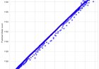
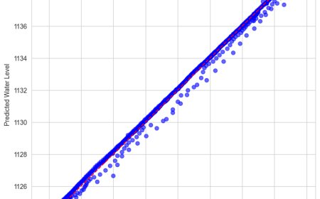
# Scatterplot of Actual vs Predicted
plt.figure(figsize=(8, 8))
plt.scatter(actual_unscaled, predicted_unscaled, alpha=0.6, color="blue")
plt.plot([min(actual_unscaled), max(actual_unscaled)], [min(actual_unscaled), max(actual_unscaled)], color="red", linestyle="--", label="Perfect Prediction")
plt.xlabel("Actual Water Level")
plt.ylabel("Predicted Water Level")
plt.title("Actual vs Predicted Water Levels")
plt.legend()
plt.show()
Let’s draw the scattered plot of actual vs predicted values Scatterplot of Actual vs Predicted

Let’s print the actual value and the predicted value of top 30 vaules side by side and see.
# Compare the predicted value vs actual value
comparison_df = pd.DataFrame({
    "Date": data["Date"][-len(actual_unscaled):],
    "Actual": actual_unscaled.flatten(),
    "Predicted": predicted_unscaled.flatten()
})
print(comparison_df.head(30))
Date Actual Predicted
3365 2010–09–27 1136.65 1137.565063
3366 2010–09–28 1136.72 1137.622070
3367 2010–09–29 1136.72 1137.656128
3368 2010–09–30 1136.80 1137.669189
3369 2010–10–01 1136.85 1137.664062
3370 2010–10–02 1136.89 1137.643433
3371 2010–10–03 1136.91 1137.609985
3372 2010–10–04 1136.91 1137.565796
3373 2010–10–05 1136.95 1137.512939
3374 2010–10–06 1136.96 1137.453735
3375 2010–10–07 1136.96 1137.393921
3376 2010–10–08 1136.95 1137.333130
3377 2010–10–09 1136.96 1137.271240
3378 2010–10–10 1136.93 1137.209839
3379 2010–10–11 1136.90 1137.150146
3380 2010–10–12 1136.87 1137.092529
3381 2010–10–13 1136.83 1137.037476
3382 2010–10–14 1136.80 1136.984863
3383 2010–10–15 1136.75 1136.934692
3384 2010–10–16 1136.72 1136.886475
3385 2010–10–17 1136.70 1136.840210
3386 2010–10–18 1136.68 1136.795654
3387 2010–10–19 1136.68 1136.753174
3388 2010–10–20 1136.64 1136.713257
3389 2010–10–21 1136.60 1136.676147
3390 2010–10–22 1136.56 1136.641479
3391 2010–10–23 1136.52 1136.609131
3392 2010–10–24 1136.48 1136.578369
3393 2010–10–25 1136.45 1136.549072
3394 2010–10–26 1136.42 1136.520508
Let’s predict the future 30 days of the water level
# Define future prediction steps (30 days of daily data)
future_steps = 30

# Start prediction from the last available data point
future_input = dataset[-look_back:]  # Use the last `look_back` data points

# Generate predictions iteratively
predictions = []
for _ in range(future_steps):
    # Predict the next step
    future_pred = model.predict(future_input.reshape(1, look_back, 1))
    predictions.append(future_pred[0, 0])
    # Update the input with the latest prediction
    future_input = np.append(future_input[1:], future_pred, axis=0)

# Inverse transform predictions to original scale
future_predictions = scaler.inverse_transform(np.array(predictions).reshape(-1, 1))

# Generate future dates
last_date = data["Date"].iloc[-1]
future_dates = pd.date_range(last_date, periods=future_steps, freq="D")

# Plot the predictions
plt.figure(figsize=(14, 7))
plt.plot(future_dates, future_predictions, label="5-Year Forecast", color="red")
plt.xlabel("Date")
plt.ylabel("Water Level")
plt.title("Tekeze 1-Year Water Level Forecast")
plt.legend()
plt.show()
Let’s the graph

That’s all. To summarize, the Deep Neural Networks have become powerful tools for businesses, enabling them to simplify complex processes and make informed decisions. These networks help analyze and identify risks, develop effective mitigation strategies, and optimize existing resources to achieve maximum output. Deep neural networks such as GRU and LSTM are excellent in predicting future from the time series data, however, the models are highly dependent on the data quality, parameters and the hyperparameters.
What's Your Reaction?